59. The Income Fluctuation Problem III: The Endogenous Grid Method#
59.1. Overview#
In this lecture we continue examining a version of the IFP from
The Income Fluctuation Problem I: Discretization and VFI and
The Income Fluctuation Problem II: Optimistic Policy Iteration.
We will make three changes.
Add a transient shock component to labor income (as well as a persistent one).
Change the timing to one that is more efficient for our set up.
Use the endogenous grid method (EGM) to solve the model.
We use EGM because we know it to be fast and accurate from Optimal Savings VI: EGM with JAX.
In addition to what’s in Anaconda, this lecture will need the following libraries:
!pip install quantecon jax
We’ll also need the following imports:
import matplotlib.pyplot as plt
import numpy as np
import numba
from quantecon import MarkovChain
import jax
import jax.numpy as jnp
from typing import NamedTuple
We will use 64-bit precision in JAX because we want to compare NumPy outputs with JAX outputs and NumPy arrays default to 64 bits.
jax.config.update("jax_enable_x64", True)
59.1.1. References#
The primary source for the technical details discussed below is [Ma et al., 2020].
Other references include [Deaton, 1991], [Den Haan, 2010], [Kuhn, 2013], [Rabault, 2002], [Reiter, 2009] and [Schechtman and Escudero, 1977].
59.2. The Household Problem#
Let’s write down the model and then discuss how to solve it.
59.2.1. Set-Up#
A household chooses a state-contingent consumption plan \(\{c_t\}_{t \geq 0}\) to maximize
subject to
Here
\(\beta \in (0,1)\) is the discount factor
\(a_t\) is asset holdings at time \(t\), with borrowing constraint \(a_t \geq 0\)
\(c_t\) is consumption
\(Y_t\) is non-capital income (wages, unemployment compensation, etc.)
\(R := 1 + r\), where \(r > 0\) is the interest rate on savings
The timing here is as follows:
At the start of period \(t\), the household observes current asset holdings \(a_t\).
The household chooses current consumption \(c_t\).
Savings \(s_t := a_t - c_t\) earns interest at rate \(r\).
Labor income \(Y_{t+1}\) is realized and time shifts to \(t+1\).
Non-capital income \(Y_t\) is given by \(Y_t = y(Z_t, \eta_t)\), where
\(\{Z_t\}\) is an exogenous state process (persistent component),
\(\{\eta_t\}\) is an IID shock process, and
\(y\) is a function taking values in \(\mathbb{R}_+\).
Throughout this lecture, we assume that \(\eta_t \sim N(0, 1)\).
We take \(\{Z_t\}\) to be a finite state Markov chain taking values in \(\mathsf Z\) with Markov matrix \(\Pi\).
The shock process \(\{\eta_t\}\) is independent of \(\{Z_t\}\) and represents transient income fluctuations.
Note
In previous lectures we used the more standard household budget constraint \(a_{t+1} + c_t \leq R a_t + Y_t\).
This setup, which is pervasive in quantitative economics, was developed for discretization.
It means that the control variable is also the next period state \(a_{t+1}\), which makes it straightforward to restrict assets to a finite grid.
But fixing the control to be the next period state forces us to include more information in the current state, which expands the size of the state space.
Moreover, aiming for discretization is not always a good idea, since it suffers heavily from the curse of dimensionality.
The timing we use here is considerably more efficient than the traditional one.
The transient component of labor income is automatially integrated out, instead of becoming a state variables.
Forcing the next period state to be the control variable is not necessary due to the use of EGM.
We further assume that
\(\beta R < 1\)
\(u\) is smooth, strictly increasing and strictly concave with \(\lim_{c \to 0} u'(c) = \infty\) and \(\lim_{c \to \infty} u'(c) = 0\)
\(y(z, \eta) = \exp(a_y \eta + z b_y)\) where \(a_y, b_y\) are positive constants
The asset space is \(\mathbb R_+\) and the state is the pair \((a,z) \in \mathsf S := \mathbb R_+ \times \mathsf Z\).
A feasible consumption path from \((a,z) \in \mathsf S\) is a consumption sequence \(\{c_t\}\) such that \(\{c_t\}\) and its induced asset path \(\{a_t\}\) satisfy
\((a_0, z_0) = (a, z)\)
the feasibility constraints in (59.1), and
adaptedness, which means that \(c_t\) is a function of random outcomes up to date \(t\) but not after.
The meaning of the third point is just that consumption at time \(t\) cannot be a function of outcomes are yet to be observed.
In fact, for this problem, consumption can be chosen optimally by taking it to be contingent only on the current state.
Optimality is defined below.
59.2.2. Value Function and Euler Equation#
The value function \(V \colon \mathsf S \to \mathbb{R}\) is defined by
where the maximization is overall feasible consumption paths from \((a,z)\).
An optimal consumption path from \((a,z)\) is a feasible consumption path from \((a,z)\) that maximizes (57.1).
To pin down such paths we can use a version of the Euler equation, which in the present setting is
with
When \(c_t\) hits the upper bound \(a_t\), the strict inequality \(u' (c_t) > \beta R \, \mathbb{E}_t u'(c_{t+1})\) can occur because \(c_t\) cannot increase sufficiently to attain equality.
The case \(c_t = 0\) never arises along the optimal path because \(u'(0) = \infty\).
59.2.3. Optimality Results#
As shown in [Ma et al., 2020],
For each \((a,z) \in \mathsf S\), a unique optimal consumption path from \((a,z)\) exists
This path is the unique feasible path from \((a,z)\) satisfying the Euler equations (59.3)-(59.4) and the transversality condition
Moreover, there exists an optimal consumption policy \(\sigma^* \colon \mathsf S \to \mathbb R_+\) such that the path from \((a,z)\) generated by
satisfies both the Euler equations (59.3)-(59.4) and (59.5), and hence is the unique optimal path from \((a,z)\).
Thus, to solve the optimization problem, we need to compute the policy \(\sigma^*\).
59.3. Computation#
We solve for the optimal consumption policy using time iteration and the endogenous grid method, which were previously discussed in
59.3.1. Solution Method#
We rewrite (59.4) to make it a statement about functions rather than random variables:
Here
\((u' \circ \sigma)(s) := u'(\sigma(s))\),
primes indicate next period states (as well as derivatives),
\(\phi\) is the density of the shock \(\eta_t\) (standard normal), and
\(\sigma\) is the unknown function.
The equality (59.6) holds at all interior choices, meaning \(\sigma(a, z) < a\).
We aim to find a fixed point \(\sigma\) of (59.6).
To do so we use the EGM.
Below we use the relationships \(a_t = c_t + s_t\) and \(a_{t+1} = R s_t + Y_{t+1}\).
We begin with an exogenous savings grid \(s_0 < s_1 < \cdots < s_m\) with \(s_0 = 0\).
We fix a current guess of the policy function \(\sigma\).
For each exogenous savings level \(s_i\) with \(i \geq 1\) and current state \(z_j\), we set
The Euler equation holds here because \(i \geq 1\) implies \(s_i > 0\) and hence consumption is interior.
For the boundary case \(s_0 = 0\) we set
We then obtain a corresponding endogenous grid of current assets via
Notice that, for each \(j\), we have \(a^e_{0j} = c_{0j} = 0\).
This anchors the interpolation at the correct value at the origin, since, without borrowing, consumption is zero when assets are zero.
Our next guess of the policy function, which we write as \(K\sigma\), is the linear interpolation of the interpolation points
for each \(j\).
(The number of one-dimensional linear interpolations is equal to the size of \(\mathsf Z\).)
59.4. NumPy Implementation#
In this section we’ll code up a NumPy version of the code that aims only for clarity, rather than efficiency.
Once we have it working, we’ll produce a JAX version that’s far more efficient and check that we obtain the same results.
We use the CRRA utility specification
Here are the utility-related functions:
@numba.jit
def u_prime(c, γ):
    return c**(-γ)

@numba.jit
def u_prime_inv(c, γ):
    return c**(-1/γ)
59.4.1. Set Up#
Here we build a class called IFPNumPy that stores the model primitives.
The exogenous state process \(\{Z_t\}\) defaults to a two-state Markov chain with transition matrix \(\Pi\).
class IFPNumPy(NamedTuple):
    R: float                  # Gross interest rate R = 1 + r
    β: float                  # Discount factor
    γ: float                  # Preference parameter
    Π: np.ndarray             # Markov matrix for exogenous shock
    z_grid: np.ndarray        # Markov state values for Z_t
    s: np.ndarray             # Exogenous savings grid
    a_y: float                # Scale parameter for Y_t
    b_y: float                # Additive parameter for Y_t
    η_draws: np.ndarray       # Draws of innovation η for MC


def create_ifp(r=0.01,
               β=0.96,
               γ=1.5,
               Π=((0.6, 0.4),
                  (0.05, 0.95)),
               z_grid=(-10.0, np.log(2.0)),
               savings_grid_max=16,
               savings_grid_size=50,
               a_y=0.2,
               b_y=0.5,
               shock_draw_size=100,
               seed=1234):

    np.random.seed(seed)
    s = np.linspace(0, savings_grid_max, savings_grid_size)
    Π, z_grid = np.array(Π), np.array(z_grid)
    R = 1 + r
    η_draws = np.random.randn(shock_draw_size)
    assert R * β < 1, "Stability condition violated."
    return IFPNumPy(R, β, γ, Π, z_grid, s, a_y, b_y, η_draws)
59.4.2. Solver#
Here is the operator \(K\) that transforms current guess \(\sigma\) into next period guess \(K\sigma\).
In practice, it takes in
a guess of optimal consumption values \(c_{ij}\), stored as
c_valsand a corresponding set of endogenous grid points \(a^e_{ij}\), stored as
ae_vals
These are converted into a consumption policy \(a \mapsto \sigma(a, z_j)\) by linear interpolation of \((a^e_{ij}, c_{ij})\) over \(i\) for each \(j\).
When we compute consumption in (59.7), we will use Monte Carlo over \(\eta'\), so that the expression becomes
with each \(\eta_{\ell}\) being a standard normal draw.
@numba.jit
def K_numpy(
        c_vals: np.ndarray,   # Initial guess of σ on grid endogenous grid
        ae_vals: np.ndarray,  # Initial endogenous grid
        ifp_numpy: IFPNumPy
    ) -> np.ndarray:
    """
    The Euler equation operator for the IFP model using the
    Endogenous Grid Method.

    This operator implements one iteration of the EGM algorithm to
    update the consumption policy function.

    """
    R, β, γ, Π, z_grid, s, a_y, b_y, η_draws = ifp_numpy
    n_a = len(s)
    n_z = len(z_grid)

    # Utility functions
    def u_prime(c):
        return c**(-γ)

    def u_prime_inv(c):
        return c**(-1/γ)

    def y(z, η):
        return np.exp(a_y * η + z * b_y)

    new_c_vals = np.zeros_like(c_vals)

    for i in range(1, n_a):  # Start from 1 for positive savings levels
        for j in range(n_z):

            # Compute Σ_z' ∫ u'(σ(R s_i + y(z', η'), z')) φ(η') dη' Π[z_j, z']
            expectation = 0.0
            for k in range(n_z):
                z_prime = z_grid[k]
                # Integrate over η draws (Monte Carlo)
                inner_sum = 0.0
                for η in η_draws:
                    # Calculate next period assets
                    next_a = R * s[i] + y(z_prime, η)
                    # Interpolate to get σ(R s_i + y(z', η), z')
                    next_c = np.interp(next_a, ae_vals[:, k], c_vals[:, k])
                    # Add to the inner sum
                    inner_sum += u_prime(next_c)
                # Average over η draws to approximate the integral
                # ∫ u'(σ(R s_i + y(z', η'), z')) φ(η') dη' when z' = z_grid[k]
                inner_mean_k = (inner_sum / len(η_draws))
                # Weight by transition probability and add to the expectation
                expectation += inner_mean_k * Π[j, k]

            # Calculate updated c_{ij} values
            new_c_vals[i, j] = u_prime_inv(β * R * expectation)

    new_ae_vals = new_c_vals + s[:, None]

    return new_c_vals, new_ae_vals
To solve the model we use a simple while loop.
def solve_model_numpy(
        ifp_numpy: IFPNumPy,
        ae_vals_init: np.ndarray,
        c_vals_init: np.ndarray,
        tol: float = 1e-5,
        max_iter: int = 1_000
    ) -> np.ndarray:
    """
    Solve the model using time iteration with EGM.

    """
    c_vals, ae_vals = c_vals_init, ae_vals_init
    i = 0
    error = tol + 1

    while error > tol and i < max_iter:
        new_c_vals, new_ae_vals = K_numpy(c_vals, ae_vals, ifp_numpy)
        error = np.max(np.abs(new_c_vals - c_vals))
        i = i + 1
        c_vals, ae_vals = new_c_vals, new_ae_vals

    return c_vals, ae_vals
Let’s road test the EGM code.
ifp_numpy = create_ifp()
R, β, γ, Π, z_grid, s, a_y, b_y, η_draws = ifp_numpy
# Initial conditions -- agent consumes everything
ae_vals_init = s[:, None] * np.ones(len(z_grid))
c_vals_init = ae_vals_init
# Solve from these initial conditions
c_vals, ae_vals = solve_model_numpy(
    ifp_numpy, c_vals_init, ae_vals_init
)
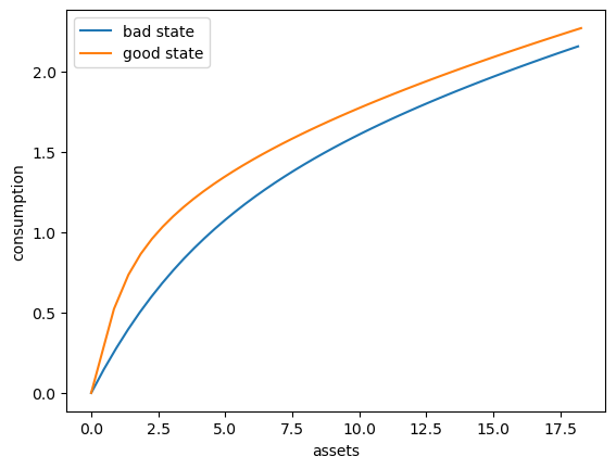
Here’s a plot of the optimal consumption policy for each \(z\) state
fig, ax = plt.subplots()

ax.plot(ae_vals[:, 0], c_vals[:, 0], label='bad state')
ax.plot(ae_vals[:, 1], c_vals[:, 1], label='good state')
ax.set(xlabel='assets', ylabel='consumption')
ax.legend()
plt.show()
59.5. JAX Implementation#
Now we write a more efficient JAX version, which can run on a GPU.
59.5.1. Set Up#
We start with a class called IFP that stores the model primitives.
class IFP(NamedTuple):
    R: float                  # Gross interest rate R = 1 + r
    β: float                  # Discount factor
    γ: float                  # Preference parameter
    Π: jnp.ndarray            # Markov matrix for exogenous shock
    z_grid: jnp.ndarray       # Markov state values for Z_t
    s: jnp.ndarray            # Exogenous savings grid
    a_y: float                # Scale parameter for Y_t
    b_y: float                # Additive parameter for Y_t
    η_draws: jnp.ndarray      # Draws of innovation η for MC


def create_ifp(r=0.01,
               β=0.96,
               γ=1.5,
               Π=((0.6, 0.4),
                  (0.05, 0.95)),
               z_grid=(-10.0, jnp.log(2.0)),
               savings_grid_max=16,
               savings_grid_size=50,
               a_y=0.2,
               b_y=0.5,
               shock_draw_size=100,
               seed=1234):

    key = jax.random.PRNGKey(seed)
    s = jnp.linspace(0, savings_grid_max, savings_grid_size)
    Π, z_grid = jnp.array(Π), jnp.array(z_grid)
    R = 1 + r
    η_draws = jax.random.normal(key, (shock_draw_size,))
    assert R * β < 1, "Stability condition violated."
    return IFP(R, β, γ, Π, z_grid, s, a_y, b_y, η_draws)
W1126 11:39:25.751007    2556 cuda_executor.cc:1802] GPU interconnect information not available: INTERNAL: NVML doesn't support extracting fabric info or NVLink is not used by the device.
W1126 11:39:25.754536    2493 cuda_executor.cc:1802] GPU interconnect information not available: INTERNAL: NVML doesn't support extracting fabric info or NVLink is not used by the device.
59.5.2. Solver#
Here is the operator \(K\) that transforms current guess \(\sigma\) into next period guess \(K\sigma\).
def K(
        c_vals: jnp.ndarray,
        ae_vals: jnp.ndarray,
        ifp: IFP
    ) -> jnp.ndarray:
    """
    The Euler equation operator for the IFP model using the
    Endogenous Grid Method.

    This operator implements one iteration of the EGM algorithm to
    update the consumption policy function.

    """
    R, β, γ, Π, z_grid, s, a_y, b_y, η_draws = ifp
    n_a = len(s)
    n_z = len(z_grid)

    # Utility functions
    def u_prime(c):
        return c**(-γ)

    def u_prime_inv(c):
        return c**(-1/γ)

    def y(z, η):
        return jnp.exp(a_y * η + z * b_y)

    def compute_c_ij(i, j):
        " Function to compute consumption for one (i, j) pair where i >= 1. "

        # For each k (future z state), compute the integral over η
        def compute_expectation_k(k):
            z_prime = z_grid[k]

            # For each η draw, compute u'(σ(R * s_i + y(z', η), z'))
            def compute_for_eta(η):
                next_a = R * s[i] + y(z_prime, η)
                # Interpolate to get σ(R * s_i + y(z', η), z')
                next_c = jnp.interp(next_a, ae_vals[:, k], c_vals[:, k])
                # Return u'(σ(R * s_i + y(z', η), z'))
                return u_prime(next_c)

            # Average over η draws to approximate the integral
            # ∫ u'(σ(R s_i + y(z', η'), z')) φ(η') dη' when z' = z_grid[k]
            return jnp.mean(jax.vmap(compute_for_eta)(η_draws))

        # Compute expectation: Σ_k [∫ u'(σ(...)) φ(η) dη] * Π[j, k]
        expectations = jax.vmap(compute_expectation_k)(jnp.arange(n_z))
        expectation = jnp.sum(expectations * Π[j, :])

        # Invert to get consumption c_{ij} at (s_i, z_j)
        return u_prime_inv(β * R * expectation)

    # Set up index grids for vmap computation of all c_{ij}
    i_grid = jnp.arange(1, n_a)
    j_grid = jnp.arange(n_z)

    # vmap over j for each i
    compute_c_i = jax.vmap(compute_c_ij, in_axes=(None, 0))
    # vmap over i
    compute_c = jax.vmap(lambda i: compute_c_i(i, j_grid))

    # Compute consumption for i >= 1
    new_c_interior = compute_c(i_grid)  # Shape: (n_a-1, n_z)

    # For i = 0, set consumption to 0
    new_c_boundary = jnp.zeros((1, n_z))

    # Concatenate boundary and interior
    new_c_vals = jnp.concatenate([new_c_boundary, new_c_interior], axis=0)

    # Compute endogenous asset grid: a^e_{ij} = c_{ij} + s_i
    new_ae_vals = new_c_vals + s[:, None]

    return new_c_vals, new_ae_vals
Here’s a jit-accelerated iterative routine to solve the model using this operator.
@jax.jit
def solve_model(
        ifp: IFP,
        c_vals_init: jnp.ndarray,   # Initial guess of σ on grid endogenous grid
        ae_vals_init: jnp.ndarray,  # Initial endogenous grid
        tol: float = 1e-5,
        max_iter: int = 1000
    ) -> jnp.ndarray:
    """
    Solve the model using time iteration with EGM.

    """

    def condition(loop_state):
        c_vals, ae_vals, i, error = loop_state
        return (error > tol) & (i < max_iter)

    def body(loop_state):
        c_vals, ae_vals, i, error = loop_state
        new_c_vals, new_ae_vals = K(c_vals, ae_vals, ifp)
        error = jnp.max(jnp.abs(new_c_vals - c_vals))
        i += 1
        return new_c_vals, new_ae_vals, i, error

    i, error = 0, tol + 1
    initial_state = (c_vals_init, ae_vals_init, i, error)
    final_loop_state = jax.lax.while_loop(condition, body, initial_state)
    c_vals, ae_vals, i, error = final_loop_state

    return c_vals, ae_vals
59.5.3. Test run#
Let’s road test the EGM code.
ifp = create_ifp()
R, β, γ, Π, z_grid, s, a_y, b_y, η_draws = ifp
# Set initial conditions where the agent consumes everything
ae_vals_init = s[:, None] * jnp.ones(len(z_grid))
c_vals_init = ae_vals_init
# Solve starting from these initial conditions
c_vals_jax, ae_vals_jax = solve_model(ifp, c_vals_init, ae_vals_init)
To verify the correctness of our JAX implementation, let’s compare it with the NumPy version we developed earlier.
# Compare the results
max_c_diff = np.max(np.abs(np.array(c_vals) - c_vals_jax))
max_ae_diff = np.max(np.abs(np.array(ae_vals) - ae_vals_jax))

print(f"Maximum difference in consumption policy: {max_c_diff:.2e}")
print(f"Maximum difference in asset grid:        {max_ae_diff:.2e}")
Maximum difference in consumption policy: 2.36e-03
Maximum difference in asset grid:        2.36e-03
These numbers confirm that we are computing essentially the same policy using the two approaches.
(Remaining differences are mainly due to different Monte Carlo integration outcomes over relatively small samples.)
Here’s a plot of the optimal policy for each \(z\) state
fig, ax = plt.subplots()
ax.plot(ae_vals[:, 0], c_vals[:, 0], label='bad state')
ax.plot(ae_vals[:, 1], c_vals[:, 1], label='good state')
ax.set(xlabel='assets', ylabel='consumption')
ax.legend()
plt.show()
59.5.4. Dynamics#
To begin to understand the long run asset levels held by households under the default parameters, let’s look at the 45 degree diagram showing the law of motion for assets under the optimal consumption policy.
fig, ax = plt.subplots()

# Compute mean labor income at each z state
R, β, γ, Π, z_grid, s, a_y, b_y, η_draws = ifp

def y(z, η):
    return jnp.exp(a_y * η + z * b_y)

def y_bar(k):
    """
    Taking z = z_grid[k], compute an approximation to

            E_z Y' = Σ_{z'} ∫ y(z', η') φ(η') dη' Π[z, z']
    """
    # Approximate ∫ y(z', η') φ(η') dη' at given z'
    def mean_y_at_z(z_prime):
        return jnp.mean(y(z_prime, η_draws))
    # Evaluate this integral across all z'
    y_means = jax.vmap(mean_y_at_z)(z_grid)
    # Weight by transition probabilities and sum
    return jnp.sum(y_means * Π[k, :])

for k, label in zip((0, 1), ('low income', 'high income')):
    # Interpolate consumption policy on the savings grid
    c_on_grid = jnp.interp(s, ae_vals[:, k], c_vals[:, k])
    ax.plot(s, R * (s - c_on_grid) + y_bar(k) , label=label)

ax.plot(s, s, 'k--')
ax.set(xlabel='current assets', ylabel='next period assets')

ax.legend()
plt.show()
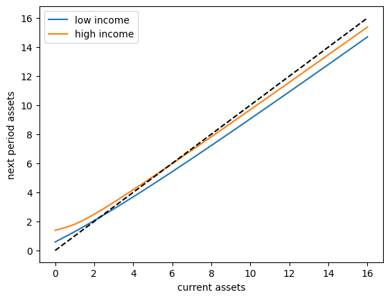
The unbroken lines show the update function for assets at each \(z\), which is
where
is a Monte Carlo approximation to expected labor income conditional on current state \(z\).
The dashed line is the 45 degree line.
The figure suggests that, on average, the dynamics will be stable — assets do not diverge even in the highest state.
This turns out to be true: there is a unique stationary distribution of assets.
For details see [Ma et al., 2020]
This stationary distribution represents the long run dispersion of assets across households when households have idiosyncratic shocks.
59.5.5. A Sanity Check#
One way to check our results is to
set labor income to zero in each state and
set the gross interest rate \(R\) to unity.
In this case, our income fluctuation problem is just a CRRA cake eating problem.
Then the value function and optimal consumption policy are given by
def c_star(x, β, γ):
    return (1 - β ** (1/γ)) * x


def v_star(x, β, γ):
    return (1 - β**(1 / γ))**(-γ) * (x**(1-γ) / (1-γ))
Let’s see if we match up:
ifp_cake_eating = create_ifp(r=0.0, z_grid=(-jnp.inf, -jnp.inf))
R, β, γ, Π, z_grid, s, a_y, b_y, η_draws = ifp_cake_eating
ae_vals_init = s[:, None] * jnp.ones(len(z_grid))
c_vals_init = ae_vals_init
c_vals, ae_vals = solve_model(ifp_cake_eating, c_vals_init, ae_vals_init)

fig, ax = plt.subplots()
ax.plot(ae_vals[:, 0], c_vals[:, 0], label='numerical')
ax.plot(ae_vals[:, 0],
        c_star(ae_vals[:, 0], ifp_cake_eating.β, ifp_cake_eating.γ),
        '--', label='analytical')
ax.set(xlabel='assets', ylabel='consumption')
ax.legend()
plt.show()
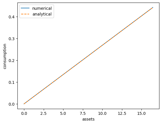
This looks pretty good.
59.6. Simulation#
Let’s return to the default model and study the stationary distribution of assets.
Our plan is to run a large number of households forward for \(T\) periods and then histogram the cross-sectional distribution of assets.
Set num_households=50_000, T=500.
First we write a function to run a single household forward in time and record the final value of assets.
The function takes a solution pair c_vals and ae_vals, understanding them
as representing an optimal policy associated with a given model ifp
@jax.jit
def simulate_household(
        key, a_0, z_idx_0, c_vals, ae_vals, ifp, T
    ):
    """
    Simulates a single household for T periods to approximate the stationary
    distribution of assets.

    - key is the state of the random number generator
    - ifp is an instance of IFP
    - c_vals, ae_vals are the optimal consumption policy, endogenous grid for ifp

    """
    R, β, γ, Π, z_grid, s, a_y, b_y, η_draws = ifp
    n_z = len(z_grid)

    def y(z, η):
        return jnp.exp(a_y * η + z * b_y)

    # Create interpolation function for consumption policy
    σ = lambda a, z_idx: jnp.interp(a, ae_vals[:, z_idx], c_vals[:, z_idx])

    # Simulate forward T periods
    def update(t, state):
        a, z_idx = state
        # Draw next shock z' from Π[z, z']
        current_key = jax.random.fold_in(key, 2*t)
        z_next_idx = jax.random.choice(current_key, n_z, p=Π[z_idx]).astype(jnp.int32)
        z_next = z_grid[z_next_idx]
        # Draw η shock
        η_key = jax.random.fold_in(key, 2*t + 1)
        η = jax.random.normal(η_key)
        # Update assets: a' = R * (a - c) + Y'
        a_next = R * (a - σ(a, z_idx)) + y(z_next, η)
        # Return updated state
        return a_next, z_next_idx

    initial_state = a_0, z_idx_0
    final_state = jax.lax.fori_loop(0, T, update, initial_state)
    a_final, _ = final_state
    return a_final
Now we write a function to simulate many households in parallel.
def compute_asset_stationary(
        c_vals, ae_vals, ifp, num_households=50_000, T=500, seed=1234
    ):
    """
    Simulates num_households households for T periods to approximate
    the stationary distribution of assets.

    Returns the final cross-section of asset holdings.

    - ifp is an instance of IFP
    - c_vals, ae_vals are the optimal consumption policy and endogenous grid.

    """
    R, β, γ, Π, z_grid, s, a_y, b_y, η_draws = ifp
    n_z = len(z_grid)

    # Create interpolation function for consumption policy
    # Interpolate on the endogenous grid
    σ = lambda a, z_idx: jnp.interp(a, ae_vals[:, z_idx], c_vals[:, z_idx])

    # Start with assets = savings_grid_max / 2
    a_0_vector = jnp.full(num_households, s[-1] / 2)
    # Initialize the exogenous state of each household
    z_idx_0_vector = jnp.zeros(num_households).astype(jnp.int32)

    # Vectorize over many households
    key = jax.random.PRNGKey(seed)
    keys = jax.random.split(key, num_households)
    # Vectorize simulate_household in (key, a_0, z_idx_0)
    sim_all_households = jax.vmap(
        simulate_household, in_axes=(0, 0, 0, None, None, None, None)
    )
    assets = sim_all_households(keys, a_0_vector, z_idx_0_vector, c_vals, ae_vals, ifp, T)

    return np.array(assets)
Now we call the function, generate the asset distribution and histogram it:
ifp = create_ifp()
R, β, γ, Π, z_grid, s, a_y, b_y, η_draws = ifp
ae_vals_init = s[:, None] * jnp.ones(len(z_grid))
c_vals_init = ae_vals_init
c_vals, ae_vals = solve_model(ifp, c_vals_init, ae_vals_init)
assets = compute_asset_stationary(c_vals, ae_vals, ifp)

fig, ax = plt.subplots()
ax.hist(assets, bins=20, alpha=0.5, density=True)
ax.set(xlabel='assets')
plt.show()
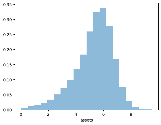
The asset distribution now shows more realistic features compared to the simple model without transient income shocks.
The addition of the IID income shock \(\eta_t\) creates more income volatility, which induces households to save more for precautionary reasons.
This helps generate more wealth inequality compared to a model with only the Markov component.
59.7. Wealth Inequality#
In this section we examine wealth inequality in more detail by computing standard measures of inequality and examining how they vary with the interest rate.
59.7.1. Measuring Inequality#
We’ll compute two common measures of wealth inequality:
Gini coefficient: A measure of inequality ranging from 0 (perfect equality) to 1 (perfect inequality)
Top 1% wealth share: The fraction of total wealth held by the richest 1% of households
Here are functions to compute these measures:
def gini_coefficient(x):
    """
    Compute the Gini coefficient for array x.

    The Gini coefficient is a measure of inequality that ranges from
    0 (perfect equality) to 1 (perfect inequality).
    """
    x = jnp.asarray(x)
    n = len(x)
    # Sort values
    x_sorted = jnp.sort(x)
    # Compute Gini coefficient
    cumsum = jnp.cumsum(x_sorted)
    return (2 * jnp.sum((jnp.arange(1, n+1)) * x_sorted)) / (n * cumsum[-1]) - (n + 1) / n


def top_share(x, p=0.01):
    """
    Compute the share of total wealth held by the top p fraction of households.

    Parameters:
        x: array of wealth values
        p: fraction of top households (default 0.01 for top 1%)

    Returns:
        Share of total wealth held by top p fraction
    """
    x = jnp.asarray(x)
    x_sorted = jnp.sort(x)
    # Number of households in top p%
    n_top = int(jnp.ceil(len(x) * p))
    # Wealth held by top p%
    wealth_top = jnp.sum(x_sorted[-n_top:])
    # Total wealth
    wealth_total = jnp.sum(x_sorted)
    return wealth_top / wealth_total if wealth_total > 0 else 0.0
Let’s compute these measures for our baseline simulation:
gini = gini_coefficient(assets)
top1 = top_share(assets, p=0.01)

print(f"Gini coefficient: {gini:.4f}")
print(f"Top 1% wealth share: {top1:.4f}")
Gini coefficient: 0.1455
Top 1% wealth share: 0.0154
These numbers are a long way out, at least for a country such as the US!
Recent numbers suggest that
the Gini coefficient for wealth in the US is around 0.8
the top 1% wealth share is over 0.3
In a later lecture we’ll see if we can improve on these numbers.
59.7.2. Interest Rate and Inequality#
Let’s examine how wealth inequality varies with the interest rate \(r\).
Economic intuition suggests that higher interest rates might increase wealth inequality, as wealthier households benefit more from returns on their assets.
Let’s investigate empirically:
# Test over 8 interest rate values
M = 8
r_vals = np.linspace(0, 0.015, M)

gini_vals = []
top1_vals = []

# Solve and simulate for each r
for r in r_vals:
    print(f'Analyzing inequality at r = {r:.4f}')
    ifp = create_ifp(r=r)
    R, β, γ, Π, z_grid, s, a_y, b_y, η_draws = ifp
    ae_vals_init = s[:, None] * jnp.ones(len(z_grid))
    c_vals_init = ae_vals_init
    c_vals, ae_vals = solve_model(ifp, c_vals_init, ae_vals_init)
    assets = compute_asset_stationary(
        c_vals, ae_vals, ifp, num_households=50_000, T=500
    )
    gini = gini_coefficient(assets)
    top1 = top_share(assets, p=0.01)
    gini_vals.append(gini)
    top1_vals.append(top1)
    # Use last solution as initial conditions for the policy solver
    c_vals_init = c_vals
    ae_vals_init = ae_vals
Analyzing inequality at r = 0.0000
Analyzing inequality at r = 0.0021
Analyzing inequality at r = 0.0043
Analyzing inequality at r = 0.0064
Analyzing inequality at r = 0.0086
Analyzing inequality at r = 0.0107
Analyzing inequality at r = 0.0129
Analyzing inequality at r = 0.0150
Now let’s visualize the results:
fig, axes = plt.subplots(1, 2, figsize=(12, 4))

# Plot Gini coefficient vs interest rate
axes[0].plot(r_vals, gini_vals, 'o-')
axes[0].set_xlabel('interest rate $r$')
axes[0].set_ylabel('Gini coefficient')
axes[0].set_title('Wealth Inequality vs Interest Rate')
axes[0].grid(alpha=0.3)

# Plot top 1% share vs interest rate
axes[1].plot(r_vals, top1_vals, 'o-', color='C1')
axes[1].set_xlabel('interest rate $r$')
axes[1].set_ylabel('top 1% wealth share')
axes[1].set_title('Top 1% Wealth Share vs Interest Rate')
axes[1].grid(alpha=0.3)

plt.tight_layout()
plt.show()
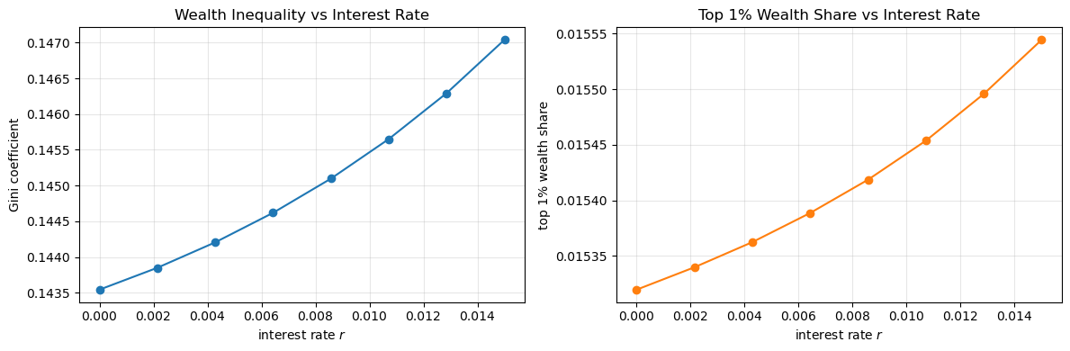
The results show that these two inequality measures increase with the interest rate.
However the differences are very minor!
Certainly changing the interest rate will not produce the kinds of numbers that we see in the data.
59.8. Exercises#
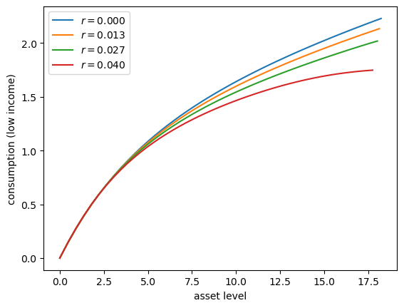
Exercise 59.1
Let’s consider how the interest rate affects consumption.
Step
rthroughnp.linspace(0, 0.016, 4).Other than
r, hold all parameters at their default values.Plot consumption against assets for income shock fixed at the smallest value.
Your figure should show that, for this model, higher interest rates suppress consumption (because they encourage more savings).
Solution
Here’s one solution:
# With β=0.96, we need R*β < 1, so r < 0.0416
r_vals = np.linspace(0, 0.04, 4)

fig, ax = plt.subplots()
for r_val in r_vals:
    ifp = create_ifp(r=r_val)
    R, β, γ, Π, z_grid, s, a_y, b_y, η_draws = ifp
    ae_vals_init = s[:, None] * jnp.ones(len(z_grid))
    c_vals_init = ae_vals_init
    c_vals, ae_vals = solve_model(ifp, c_vals_init, ae_vals_init)
    # Plot policy
    ax.plot(ae_vals[:, 0], c_vals[:, 0], label=f'$r = {r_val:.3f}$')
    # Start next round with last solution
    c_vals_init = c_vals
    ae_vals_init = ae_vals

ax.set(xlabel='asset level', ylabel='consumption (low income)')
ax.legend()
plt.show()
Exercise 59.2
Following on from Exercises 1, let’s look at how savings and aggregate asset holdings vary with the interest rate
Note
[Ljungqvist and Sargent, 2018] section 18.6 can be consulted for more background on the topic treated in this exercise.
For a given parameterization of the model, the mean of the stationary distribution of assets can be interpreted as aggregate capital in an economy with a unit mass of ex-ante identical households facing idiosyncratic shocks.
Your task is to investigate how this measure of aggregate capital varies with the interest rate.
Intuition suggests that a higher interest rate should encourage capital formation — test this.
For the interest rate grid, use
M = 8
r_vals = np.linspace(0, 0.015, M)
Solution
Here’s one solution
fig, ax = plt.subplots()

asset_mean = []
for r in r_vals:
    print(f'Solving model at r = {r}')
    ifp = create_ifp(r=r)
    R, β, γ, Π, z_grid, s, a_y, b_y, η_draws = ifp
    ae_vals_init = s[:, None] * jnp.ones(len(z_grid))
    c_vals_init = ae_vals_init
    c_vals, ae_vals = solve_model(ifp, c_vals_init, ae_vals_init)
    assets = compute_asset_stationary(c_vals, ae_vals, ifp, num_households=10_000, T=500)
    mean = np.mean(assets)
    asset_mean.append(mean)
    print(f'  Mean assets: {mean:.4f}')
    # Start next round with last solution
    c_vals_init = c_vals
    ae_vals_init = ae_vals
ax.plot(r_vals, asset_mean)

ax.set(xlabel='interest rate', ylabel='capital')

plt.show()
Solving model at r = 0.0
  Mean assets: 4.7290
Solving model at r = 0.002142857142857143
  Mean assets: 4.8296
Solving model at r = 0.004285714285714286
  Mean assets: 4.9380
Solving model at r = 0.006428571428571429
  Mean assets: 5.0553
Solving model at r = 0.008571428571428572
  Mean assets: 5.1828
Solving model at r = 0.010714285714285714
  Mean assets: 5.3222
Solving model at r = 0.012857142857142859
  Mean assets: 5.4756
Solving model at r = 0.015
  Mean assets: 5.6452
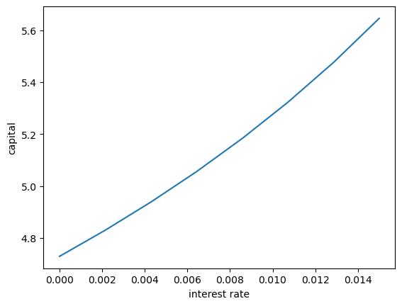
As expected, aggregate savings increases with the interest rate.